
Model Description
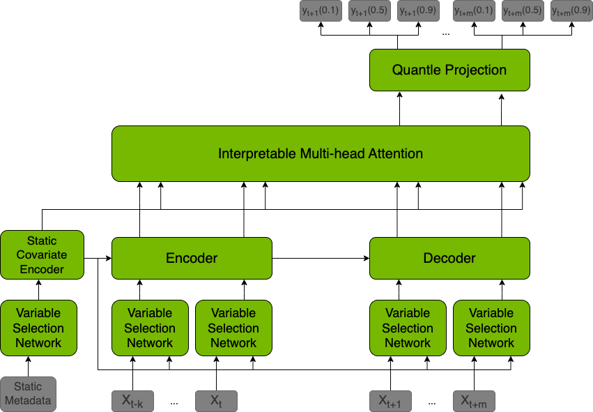
The Temporal Fusion Transformer TFT model is a state-of-the-art architecture for interpretable, multi-horizon time-series prediction. The model was first developed and implemented by Google with the collaboration with the University of Oxford.
This implementation differs from the reference implementation by addressing the issue of missing data, which is common in production datasets, by either masking their values in attention matrices or embedding them as a special value in the latent space.
This model enables the prediction of confidence intervals for future values of time series for multiple future timesteps.
Example
In the following example, we will use the pretrained TFT model to perform inference on some preprocessed samples from the Electricity dataset. To run the example, you need some extra python packages installed for loading and visualization.
!pip install scikit-learn==1.2.1
!pip install pandas==1.5.3
!pip install matplotlib==3.6.3
import torch
import os
import numpy as np
import matplotlib.pyplot as plt
import pickle
from mpl_toolkits.axes_grid1 import make_axes_locatable
import warnings
warnings.filterwarnings('ignore')
os.environ["TFT_SCRIPTING"] = "True"
if torch.cuda.is_available():
    device = torch.device("cuda")
    !nvidia-smi
else:
    device = torch.device("cpu")
print(f'Using {device} for inference')
Load the model pretrained on the Electricity dataset.
tft_model = torch.hub.load("../../../../public", "nvidia_tft", dataset="electricity", pretrained=True, source="local")
utils = torch.hub.load("../../../../public", "nvidia_tft_data_utils", source="local")
Download and preprocess the data. This can take a few minutes.
utils.download_data(torch.hub._get_torch_home())
utils.preprocess(torch.hub._get_torch_home())
Initialize functions used to get interpretable attention graphs.
activations = {}
def get_attention_heatmap_fig(heads, max_size=16, min_size=4):
    row_size = max(min_size, max_size / len(heads))
    fig, axes = plt.subplots(1, len(heads), figsize=(max_size, row_size))
    for i, (head, ax) in enumerate(zip(heads, axes), 1):
        im = ax.imshow(head, cmap='hot', interpolation='nearest')
        if i < len(heads):
            ax.set_title(f'HEAD {i}')
        else:
            ax.set_title(f'MEAN')
            divider = make_axes_locatable(ax)
            cax = divider.append_axes('right', size='5%', pad=0.05)
            fig.colorbar(im, cax=cax, orientation='vertical')
    return fig

def get_attn_heads(activations, sample_number):
    heads = []
    _, attn_prob = activations
    sample_attn_prob = attn_prob[sample_number]
    n_heads = sample_attn_prob.shape[0]
    for head_index in range(n_heads):
        head = sample_attn_prob[head_index] * 255
        heads.append(head.detach().cpu())
    mean_head = torch.mean(sample_attn_prob, dim=0) * 255
    heads.append(mean_head.detach().cpu())
    fig = get_attention_heatmap_fig(heads)
    return fig

def _get_activation(name):
    def hook(model, input, output):
        activations[name] = output

    return hook
Register the hook on the model to save the data.
tft_model.attention.register_forward_hook(_get_activation('attention'))
Load the sample preprocessed batch of data.
batch = utils.get_batch(torch.hub._get_torch_home())
batch = {key: tensor.to(device) if tensor.numel() else None for key, tensor in batch.items()}
Run inference on the TFT.
tft_model.to(device)
tft_model.eval()
with torch.no_grad():
    output= tft_model(batch)
output.shape
batch['target'].shape
Plot the full 192 timestep window of the Electricity dataset. We use the previous week of data to predict the following day of power usage. Since our data is organized by hour, this means we use 168 previous time points to predict the following 24.
index = 9
fig, ax = plt.subplots()
ax.plot(batch['target'][index].cpu().numpy(), label="Ground Truth")
ax.plot(np.arange(168, 192), output[index].detach().cpu().numpy(), label=["10th Quantile", "50th Quantile", "90th Quantile"])
ax.legend(loc='upper left')

ax.set_xlabel('Timestep')
ax.set_ylabel('Power Usage')
Below is the same graph as above, but only focusing on the prediction window, which is the last 24 values.
fig, ax = plt.subplots()
ax.plot(np.arange(168, 192), batch['target'][index][-24:].cpu().numpy(), label="Ground Truth")
ax.plot(np.arange(168, 192), output[index].detach().cpu().numpy(), label=["10th Quantile", "50th Quantile", "90th Quantile"])
ax.legend(loc='upper left')

ax.set_xlabel('Timestep')
ax.set_ylabel('Power Usage')
Using the hook we defined earlier we can generate plots of the attention heads. There is a clear trend that more recent values are given more weight. In addition, the striations in the graphs are every 24 hours, which indicates that there is some correlation between data on the same hour of different days. Indeed, looking back on the graphs above there is a cyclical pattern to the power usage that repeats every 24 hours.
attn_graphs = get_attn_heads(activations['attention'], index)
Details
For detailed information on model input and output, training recipies, inference and performance visit: Deep Learning Examples
References
- Temporal Fusion Transformers for Interpretable Multi-horizon Time Series Forecasting
- model on github
- pretrained model on NGC (Electricity)
- pretrained model on NGC (Traffic)
